这两天温习了一下机器学习中学到的一个模型——MLP(Multilayer Perceptron)多层感知机,使用pytorch框架复现了一下虽然抄的代码以及没什么难度,借这个机会完整学习一下pytorch框架,挺有必要的
参考书籍:《动手学深度学习》以下简称d2l
pytorch是一个比较主流的构建深度学习模型的框架,深入学习才略微窥见它的强大
MLP实现
设定问题
- 使用MLP对Fashion-MNIST数据集进行十个类别的分类
解决过程
- 数据集加载
- 构建MLP模型
- 构建训练、测试过程
这里在构建MLP,定义了这样一个模块
from torch import nn

class MLP(nn.Module):
    def __init__(self, input_num):
        super(MLP, self).__init__()
        self.flatten = nn.Flatten()
        self.linear_relu_stack = nn.Sequential(
            nn.Linear(input_num, 256),
            nn.ReLU(),
            nn.Linear(256, 10),
        )

    def forward(self, x):
        x = self.flatten(x)
        pred = self.linear_relu_stack(x)
        return pred
训练函数
def train(train_iter, model, loss_fn, optimizer):
    print(f"train on {device}")

    model = model.to(device)
    size = len(train_iter.dataset)

    for batch, (X, y) in enumerate(train_iter):
        X = X.to(device)
        y = y.to(device)
        pred = model(X)
        loss = loss_fn(pred, y)

        optimizer.zero_grad()
        loss.backward()
        optimizer.step()

        if batch % 100 == 0:
            loss, current = loss.item(), batch * len(X)
            print(f"loss:{loss:>7f} [{current:>5d}/{size:>5d}]")
测试函数
def test(test_iter, model, loss_fn):
    model = model.to(device)
    size = len(test_iter.dataset)
    num_batches = len(test_iter)
    test_loss, correct = 0, 0

    with torch.no_grad():
        for X, y in test_iter:
            X = X.to(device)
            y = y.to(device)

            pred = model(X)
            test_loss += loss_fn(pred, y).item()
            correct += (pred.argmax(1) == y).type(torch.float).sum().item()

    test_loss /= num_batches

    correct /= size

    print(f"test error:\n accuracy:{(100 * correct):>0.1f}%,avg loss: {test_loss:>8f} \n")
这两个函数其实是比较套路化的
- 模型加载到设备(磁盘)中
- 数据加载到设备中
- 使用模型对输入进行计算并给出输出
- 训练过程梯度反向传播
在d2l中在深度学习计算中介绍了比较详细的步骤
模型构建、参数访问与初始化、设计自定义层和块、将模型读写到磁盘,以及利用GPU实现显著的加速
接下来就跟着d2l学习深度学习计算
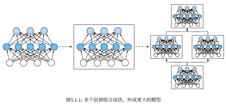
层和块
利用矢量化算法来描述整层神经元
层
- 接受一组输入
- 生成相应的输出
- 由一组可调整参数描述
块可以描述单个层、由多个层组成的组件或整个模型本身
块
由类class表示,上面的类MLP就是一个神经网络块
- 将输入数据作为其前向传播函数的参数。
- 通过前向传播函数来生成输出。
- 计算其输出关于输入的梯度,可通过其反向传播函数进行访问。通常这是自动发生的。
- 存储和访问前向传播计算所需的参数。
- 根据需要初始化模型参数。
MLP的一个简洁实现
import torch
from torch import nn
from torch.nn import functional as F

net=nn.Sequential(nn.Linear(20,256),nn.ReLU(),nn.Linear(256,10))

X=torch.rand(2,20)

print(net(X))
tensor([[-0.0117, -0.0788, 0.1455, -0.0129, -0.0806, 0.0068, -0.2311, -0.1886,
-0.0746, -0.1914],
[ 0.0570, -0.0040, 0.0808, 0.0587, -0.0073, 0.0147, -0.1427, -0.1364,
-0.1199, -0.0975]], grad_fn=<AddmmBackward0>)nn.Sequential定义了一种特殊的Module,即在PyTorch中表示一个块的类,它维护了一个由Module组成的有序列表
自定义块
简要总结一下每个块必须提供的基本功能
将输入数据作为其前向传播函数的参数。
通过前向传播函数来生成输出。请注意,输出的形状可能与输入的形状不同。例如,我们上面模型中的第一个全连接的层接收一个20维的输入,但是返回一个维度为256的输出。
计算其输出关于输入的梯度,可通过其反向传播函数进行访问。通常这是自动发生的。
存储和访问前向传播计算所需的参数。
根据需要初始化模型参数。
自定义块继承表示块的类
实现只需要提供自己的构造函数(Python中的__init__函数)和前向传播函数
吃个栗子
一个多层感知机,其具有一个20维输入层、256个隐藏单元的隐藏层和一个10维输出层
import torch
from torch import nn
from torch.nn import functional as F


class MLP(nn.Module):
    def __init__(self):
        super().__init__()
        self.hidden = nn.Linear(20, 256)
        self.out = nn.Linear(256, 10)

    def forward(self, X):
        return self.out(F.relu(self.hidden(X)))


net = MLP()
X = torch.rand(2, 20)
print(net(X))
测试一下
tensor([[-0.0367, -0.0619, -0.1407, -0.0066,  0.0359,  0.0313,  0.1103, -0.0920,
          0.0879, -0.0706],
        [ 0.0113, -0.1204, -0.1172, -0.0580,  0.0252,  0.0236,  0.0859, -0.0516,
0.1003, 0.0124]], grad_fn=<AddmmBackward0>)看着自定义应该是用的最多的毕竟可以自定义可以整花活
顺序块
Sequential类
Sequential的设计是为了把其他模块串起来
构建简化的MySequential,只需要定义两个关键函数
一种将块逐个追加到列表中的函数;
一种前向传播函数,用于将输入按追加块的顺序传递给块组成的“链条”。
在上面的MLP的一个简洁实现中就是使用了默认Sequential类
net=nn.Sequential(nn.Linear(20,256),nn.ReLU(),nn.Linear(256,10))吃个栗子
MySequential提供与默认Sequential类相同的功能
import torch
from torch import nn
from torch.nn import functional as F


class MySequential(nn.Module):
    def __init__(self, *args):
        super().__init__()
        for idx, module in enumerate(args):
            self._modules[str(idx)] = module

    def forward(self, X):
        for block in self._modules.values():
            X = block(X)

        return X


X = torch.rand(2, 20)

net = MySequential(nn.Linear(20, 256), nn.ReLU(), nn.Linear(256, 10))

print(net(X))上述代码相当于复现了nn.Sequential类
测试结果
tensor([[-0.1147, -0.1456,  0.2465,  0.0962,  0.0054,  0.0990,  0.2512,  0.1100,
         -0.1132,  0.3261],
        [-0.1703, -0.1180,  0.1107,  0.0750, -0.0046,  0.1504,  0.2909,  0.2881,
         -0.1164,  0.2153]], grad_fn=<AddmmBackward0>)
前向传播函数中执行代码
现实中的深度学习计算并不可能总是顺序块执行,也就是说需要自定义前向传播函数
吃个栗子
需要一个计算函数
$$
f(\mathbf{x},\mathbf{w})=c\cdot\mathbf{w}^{T}\mathbf{x}
$$
层,命名为FixedHiddenMLP,其中$\mathbf{w}$是参数,$\mathbf{x}$是参数,$c$是某个在优化过程中没有更新的指定常量
import torch
from torch import nn
from torch.nn import functional as F


class FixedHiddenMLP(nn.Module):
    def __init__(self):
        super().__init__()
        self.rand_weight = torch.rand((20, 20), requires_grad=False)
        self.linear = nn.Linear(20, 20)

    def forward(self, X):
        X = self.linear(X)
        X = F.relu(torch.mm(X, self.rand_weight) + 1)
        X = self.linear(X)
        return X.sum()
测试结果
tensor(0.0017, grad_fn=<SumBackward0>)小结
- 一个块可以由许多层组成;一个块可以由许多块组成。
- 块可以包含代码。
- 块负责大量的内部处理,包括参数初始化和反向传播。
- 层和块的顺序连接由Sequential块处理。
参数管理
构建模型之后,需要训练模型,也就是俗称的调参,目标是找到损失函数最小的模型参数
参数管理有以下几点:
- 访问参数
- 参数初始化
- 模型组件间共享参数
单隐藏层MLP起手
import torch
from torch import nn

net=nn.Sequential(nn.Linear(4,8),nn.ReLU(),nn.Linear(8,1))

X=torch.rand(size=(2,4))

print(net(X))
tensor([[-0.4368],
[-0.2469]], grad_fn=<AddmmBackward0>)参数访问
通过Sequential类定义模型时,我们可以通过索引来访问模型的任意层
print(net[2].state_dict())OrderedDict([('weight', tensor([[-0.2442, -0.0573, 0.3293, -0.1345, 0.1103, 0.1605, 0.0275, 0.1626]])), ('bias', tensor([0.3034]))])包括权重和偏置
目标参数
每个参数都表示为参数类的一个实例
要对参数执行任何操作,需要访问底层的数值
吃个栗子
提取以上网络中的第二个全连接层的偏置
print(type(net[2].bias))
print(net[2].bias)
print(net[2].bias.data)
<class 'torch.nn.parameter.Parameter'>
Parameter containing:
tensor([0.3034], requires_grad=True)
tensor([0.3034])参数是复合的对象,包含值、梯度和额外信息;除了值之外,还可以访问每个参数的梯度
由于还没有调用反向传播,参数的梯度处于初始状态
net[2].weight.grad is NoneTrue一次性访问所有参数
递归整个树来提取每个子块的参数
吃个栗子
访问第一个全连接层的参数和访问所有层
print(*[(name, param.shape) for name, param in net[0].named_parameters()])
print(*[(name, param.shape) for name, param in net.named_parameters()])
('weight', torch.Size([8, 4])) ('bias', torch.Size([8]))
('0.weight', torch.Size([8, 4])) ('0.bias', torch.Size([8])) ('2.weight', torch.Size([1, 8])) ('2.bias', torch.Size([1]))体现了另一种访问目标参数的方法
net.state_dict()['2.bias'].datatensor([0.3034])从嵌套块中提取参数
“块工厂”起手
def block1():
    return nn.Sequential(nn.Linear(4, 8), nn.ReLU(), nn.Linear(8, 4), nn.ReLU())


def block2():
    net = nn.Sequential()
    for i in range(4):
        net.add_module(f'block {i}', block1())
    return net


rgnet = nn.Sequential(block2(), nn.Linear(4, 1))
rgnet(X)
tensor([[-0.5041],
[-0.5041]], grad_fn=<AddmmBackward0>)查看网络结构
Sequential(
  (0): Sequential(
    (block 0): Sequential(
      (0): Linear(in_features=4, out_features=8, bias=True)
      (1): ReLU()
      (2): Linear(in_features=8, out_features=4, bias=True)
      (3): ReLU()
    )
    (block 1): Sequential(
      (0): Linear(in_features=4, out_features=8, bias=True)
      (1): ReLU()
      (2): Linear(in_features=8, out_features=4, bias=True)
      (3): ReLU()
    )
    (block 2): Sequential(
      (0): Linear(in_features=4, out_features=8, bias=True)
      (1): ReLU()
      (2): Linear(in_features=8, out_features=4, bias=True)
      (3): ReLU()
    )
    (block 3): Sequential(
      (0): Linear(in_features=4, out_features=8, bias=True)
      (1): ReLU()
      (2): Linear(in_features=8, out_features=4, bias=True)
      (3): ReLU()
    )
  )
  (1): Linear(in_features=4, out_features=1, bias=True)
)
有两大块,编号0、1
0块有四子块,编号block 0、block 1、block 2、block 3
层是分层嵌套的,可以通过嵌套列表索引访问参数
吃个栗子
访问第一个大块中第二个子块的第一层的偏置项
print(rgnet[0][1][0].bias)Parameter containing:
tensor([-0.2775, 0.4211, -0.3803, -0.3675, -0.2259, -0.3390, -0.3779, -0.4868],
requires_grad=True)参数初始化
深度学习框架提供默认随机初始化,也允许创建自定义初始化方法,通过其他规则实现初始化权重
PyTorch会根据一个范围均匀地初始化权重和偏置矩阵,这个范围是根据输入和输出维度计算出的。PyTorch的nn.init模块提供了多种预置初始化方法
内置初始化
吃个栗子
将所有权重参数初始化为标准差为0.01的高斯随机变量,且将偏置参数设置为0
def init_normal(m):
    if type(m)==nn.Linear:
        nn.init.normal_(m.weight,mean=0,std=0.01)
        nn.init.zeros_(m.bias)

net.apply(init_normal)
net[0].weight.data[0], net[0].bias.data[0]
(tensor([-0.0017, 0.0091, -0.0117, 0.0023]), tensor(0.))将所有参数初始化为给定的常数1
def init_constant(m):
    if type(m)==nn.Linear:
        nn.init.constant_(m.weight,1)
        nn.init.zeros_(m.bias)

nn.apply(init_constant)
net[0].weight.data[0], net[0].bias.data[0]
(tensor([1., 1., 1., 1.]), tensor(0.))对某些块应用不同的初始化方法
使用Xavier初始化方法初始化第一个神经网络层,然后将第三个神经网络层初始化为常量值42
def init_xavier(m):
    if type(m)==nn.Linear:
        nn.init.xavier_uniform_(m.weight)

def init_42(m):
    if type(m)==nn.Linear:
        nn.init.constant_(m.weight,42)

net[0].apply(init_xavier)
net[2].apply(init_42)
print(net[0].weight.data)
print(net[2].weight.data)
tensor([[ 0.5929, -0.6632, 0.5801, -0.3955],
[ 0.5474, -0.4001, -0.5903, -0.2604],
[-0.3803, 0.5339, -0.2067, 0.2727],
[-0.3436, 0.6771, -0.4843, -0.5433],
[ 0.4772, -0.3573, -0.3501, -0.6893],
[-0.1906, 0.1262, -0.0837, -0.0278],
[ 0.5113, -0.5042, 0.0093, 0.6083],
[-0.4959, -0.0665, -0.0333, -0.4934]])
tensor([[42., 42., 42., 42., 42., 42., 42., 42.]])自定义初始化
吃个栗子
使用以下的分布为任意权重参数$w$定义初始化方法
$$
w\sim\begin{cases}U(5,10)&\text{可能性}\frac14\[2ex]0&\text{可能性}\frac12\[2ex]U(-10,-5)&\text{可能性}\frac14\end{cases}
$$
def my_init(m):
    if type(m)==nn.Linear:
        print("Init",*[(name,param.shape) for name,param in m.named_parameters()])
        nn.init.uniform_(m.weight,-10,10)
        m.weight.data *= m.weight.data.abs()>=5

net.apply(my_init)
net[0].weight[:2]
Init weight torch.Size([8, 4])
Init weight torch.Size([1, 8])
tensor([[ 0.0000, -0.0000, -8.7441, -7.0742],
[ 5.3636, -8.9511, -8.9778, 5.7546]], grad_fn=<SliceBackward0>)参数绑定
希望在多个层间共享参数:我们可以定义一个稠密层,然后使用它的参数来设置另一个层的参数
吃个栗子
shared=nn.Linear(8,8)

net=nn.Sequential(nn.Linear(4,8),nn.ReLU(),shared,nn.ReLU(),shared,nn.ReLU(),nn.Linear(8,1))

net(X)
print(net[2].weight.data[0]==net[4].weight.data[0])

net[2].weight.data[0,0]=100

print(net[2].weight.data[0]==net[4].weight.data[0])
tensor([True, True, True, True, True, True, True, True])
tensor([True, True, True, True, True, True, True, True])第三个和第五个神经网络层的参数是绑定的
不仅值相等,而且由相同的张量表示
如果改变其中一个参数,另一个参数也会改变
当参数绑定时,梯度变化?
模型参数包含梯度,因此在反向传播期间第二个隐藏层(即第三个神经网络层)和第三个隐藏层(即第五个神经网络层)的梯度会加在一起
延后初始化
在没有得到数据的情况下就要建立网络,会遇到一些数据性的问题
- 定义了网络架构,但没有指定输入维度。
- 添加层时没有指定前一层的输出维度。
- 在初始化参数时,没有足够的信息来确定模型应该包含多少参数。
框架的延后初始化(defers initialization),即直到数据第一次通过模型传递时,框架才会动态地推断出每个层的大小。
延后初始化能够解决上面的问题
实例化网络
以MLP为例
输入维数未知,定义一个变量作为矩阵形状
def get_net(input_feature,output_feature):
    net=nn.Sequential(nn.Linear(input_feature,8),nn.ReLU(),nn.Linear(8,output_feature))
    return net

net=get_net(4,1)
print(net)
将数据通过网络,最终使框架初始化参数
自定义层
不带参数的层
构造一个没有任何参数的自定义层,只需继承基础层类并实现前向传播功能
吃个栗子
实现一个数据中心化层
import torch
import torch.nn.functional as F
from torch import nn


class CenteredLayer(nn.Module):
    def __init__(self):
        super().__init__()

    def forward(self, X):
        return X - X.mean()

layer=CenteredLayer()
layer(torch.FloatTensor([1,2,3,4,5]))
带参数的层
定义具有参数的层,这些参数可以通过训练进行调整
使用内置函数来创建参数,这些函数提供一些基本的管理功能
如管理访问、初始化、共享、保存和加载模型参数
吃个栗子
实现自定义版本的全连接层
该层需要两个参数,一个用于表示权重,另一个用于表示偏置项
使用修正线性单元ReLU作为激活函数
包括输入、输出数
class MyLinear(nn.Module):
    def __init__(self,in_units,units):
        super().__init__()
        self.weight=nn.Parameter(torch.randn(in_units,units))
        self.bias=nn.Parameter(torch.randn(units,))

    def forward(self,X):
        linear=torch.matmul(X,self.weight.data)+self.bias.data
        return F.relu(linear)

linear=MyLinear(5,3)
linear.weight
Parameter containing:
tensor([[ 1.2648, -1.2138, -0.6748],
[-0.0369, -1.0866, 0.1367],
[-1.2023, -0.7454, -1.4862],
[ 2.1399, -1.3201, -0.5928],
[-1.7694, 1.3518, 1.9013]], requires_grad=True)读写文件
定期保存中间结果
加载和存储权重向量和整个模型
加载和保存张量
对于单个张量,可以直接调用load和save函数分别读写它们
import torch
from torch import nn
from torch.nn import functional as F

x=torch.arange(4)
torch.save(x,'x-file')x2=torch.load('x-file')
x2tensor([0, 1, 2, 3])吃个栗子
存储一个张量列表,然后把它们读回内存
y=torch.zeros(4)
torch.save([x,y],'x-files')
x2,y2=torch.load('x-files')
(x2,y2)
(tensor([0, 1, 2, 3]), tensor([0., 0., 0., 0.]))写入或读取从字符串映射到张量的字典
diction={'x':x,'y':y}
torch.save(diction,'diction')
diction2=torch.load('diction')
diction2
{'x': tensor([0, 1, 2, 3]), 'y': tensor([0., 0., 0., 0.])}加载和保存模型参数
深度学习框架提供了内置函数来保存和加载整个网络
保存模型的参数而不是保存整个模型
为了恢复模型,需要用代码生成架构,然后从磁盘加载参数
吃个栗子
保存、加载MLP参数
import torch
from torch import nn

class MLP(nn.Module):
    def __init__(self):
        super().__init__()
        self.myMLP=nn.Sequential(
            nn.Linear(20,256),
            nn.ReLU(),
            nn.Linear(256,10)
        )

    def forward(self,X):
        return self.myMLP(X)

net=MLP()
X=torch.randn((2,20))
net(X)
tensor([[-0.3972, -0.0309, 0.2046, -0.3960, -0.8005, 0.1611, 0.1087, 0.5269,
0.0768, 0.2946],
[ 0.2391, 0.2807, 0.2612, 0.2114, 0.1242, -0.0763, 0.3262, 0.1143,
0.2923, -0.2082]], grad_fn=<AddmmBackward0>)torch.save(net.state_dict(),'mlp.params')clone=MLP()
clone.load_state_dict(torch.load('mlp.params'))
cloneMLP(
(myMLP): Sequential(
(0): Linear(in_features=20, out_features=256, bias=True)
(1): ReLU()
(2): Linear(in_features=256, out_features=10, bias=True)
)
)Y_clone=clone(X)
Y_clone==net(X)tensor([[True, True, True, True, True, True, True, True, True, True],
[True, True, True, True, True, True, True, True, True, True]])保存架构必须在代码中完成,而不是在参数中完成
GPU
!nvidia-smiMon Feb 26 19:20:29 2024
+---------------------------------------------------------------------------------------+
| NVIDIA-SMI 546.26 Driver Version: 546.26 CUDA Version: 12.3 |
|-----------------------------------------+----------------------+----------------------+
| GPU Name TCC/WDDM | Bus-Id Disp.A | Volatile Uncorr. ECC |
| Fan Temp Perf Pwr:Usage/Cap | Memory-Usage | GPU-Util Compute M. |
| | | MIG M. |
|=========================================+======================+======================|
| 0 NVIDIA GeForce GTX 1650 WDDM | 00000000:01:00.0 Off | N/A |
| N/A 48C P8 1W / 50W | 78MiB / 4096MiB | 0% Default |
| | | N/A |
+-----------------------------------------+----------------------+----------------------+
+---------------------------------------------------------------------------------------+
| Processes: |
| GPU GI CI PID Type Process name GPU Memory |
| ID ID Usage |
|=======================================================================================|
| 0 N/A N/A 13688 C+G D:\tecent\QQ.exe N/A |
| 0 N/A N/A 23400 C+G D:\tecent\QQ.exe N/A |
+---------------------------------------------------------------------------------------+
后面因为没有多卡就没有继续